A KPI (Key Performance Indicator) is a graphical representation that displays progress against a predefined measure or business goal. KPIs make it easier for end users to evaluate the amount of progress without reading a bunch of data.
In this post, I’ll use AdventureWorksDW2012 sample data so you can follow along with me. The database can be downloaded here.
Let’s get started.
Enabling PowerPivot in Excel 2013
To enable PowerPivot, open Excel, go to File, Options, Add-Ins, select COM Add-ins and click Go. This will open up the COM Add-Ins dialog box. Click “Microsoft Office PowerPivot for Excel 2013” and hit OK. After successfully enabling PowerPivot, the tab should appear at the top of the Excel spreadsheet:
Importing Data
Open Excel, click the PowerPivot tab, Manage:

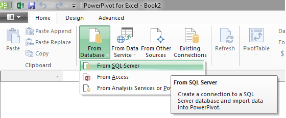
Upon clicking Manage, a new window should appear. From this window, you will import data. Click From Database and select From SQL Server:

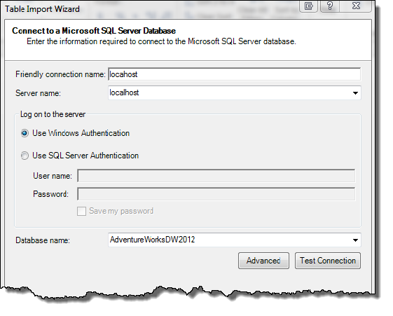
Type in the Server Name, Authentication mode, and browse to the AdventureWorksDW2012 database:
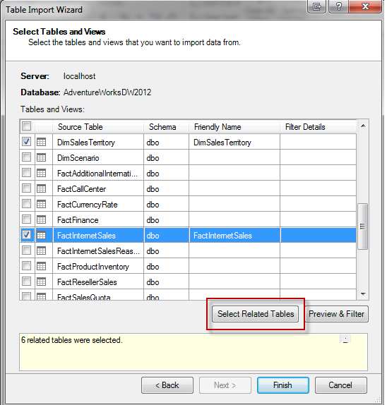
 Click Next, choose “Select from a list of tables and views to choose the data to import” and click Next. The next screen is where we will select our data to import. For this example, choose FactInternetSales and click “Select Related Tables”. The Select Related Tables button enables you to automatically select every table that is related to the source table selected:

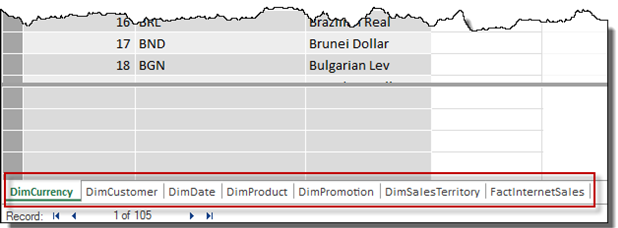
After clicking Finish, the import will begin. Once the import finishes successfully you should be able to view all the tables separated into sheets:
Creating PivotTable
Before creating a KPI we will need to slice and dice our data into a PivotTable. To do this, click PivotTable on the ribbon bar and choose New Worksheet:


